How to Build a CPG Inventory Replenishment Model (A CFO Framework for Accuracy, Cash Control & Service Levels)
A CFO-grade replenishment model integrates demand forecasting, safety stock logic, lead times, MOQs, channel behavior, and financial constraints into one system. When implemented correctly, CPG brands reduce total inventory 15 to 30%, increase fill rates above 97%, and eliminate the constant stockout firefighting cycle. Replenishment is a CFO-controlled engine, not just an operations workflow, because it directly determines cash conversion, margin performance, and working capital requirements.
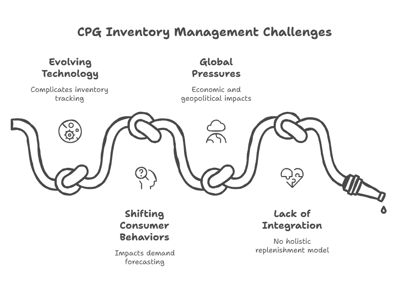
Why Most CPG Brands Get Replenishment Wrong
We worked with a snack brand doing $18M annually across grocery, convenience, and club channels. Their inventory turnover sat at 4.2x while competitors averaged 7.1x. They carried $1.4M in average inventory when the business needed closer to $850K. Finance blamed operations for over-ordering. Operations blamed finance for not understanding lead times. Sales blamed everyone for the $340K in lost revenue during Q2 peak season from stockouts on their top three SKUs.
The actual problem was simpler: they had no replenishment model. They used a spreadsheet that calculated months of supply based on last year’s sales, adjusted by gut feel for seasonality. When a major retailer buyer doubled an order, the operations team scrambled. When a promotion underperformed, they were left with excess inventory that sat for nine months and eventually generated chargebacks.
This pattern repeats across hundreds of CPG brands. Companies with sophisticated trade spend models and detailed P&L forecasts often run replenishment on instinct and reactive firefighting. The result is predictable: too much cash trapped in slow-moving inventory, frequent stockouts on fast movers, constant expedited freight charges, and a persistent sense that the business is always one week away from a service failure.
What a Real Replenishment Model Actually Does
A CFO-grade replenishment model is not a simple reorder point calculator. It is a dynamic system that answers one specific question every day for every SKU: given current inventory position, forecasted consumer demand, production constraints, and cash availability, what should we order today to optimize service levels while minimizing working capital?
The model integrates seven components that most brands either ignore entirely or manage in separate, disconnected systems.
The Seven Core Components of a CFO-Grade Replenishment Model
| Component | What It Answers | Why It Gets Ignored |
| Demand forecasting engine | How much will consumers actually buy? | Brands forecast from shipments, not POS data |
| Inventory position tracking | What do we actually have available? | In-transit and allocated inventory excluded |
| Safety stock logic | How much buffer per SKU? | Flat rules applied regardless of variability |
| Lead time management | When do we need to order? | Production variability not modeled |
| MOQ and production constraints | What can we actually order? | Co-packer minimums handled ad hoc |
| Channel-specific behavior | How does each channel order? | One logic applied to all channels |
| Cash flow constraints | What can we afford right now? | Finance and operations not connected |
Building the Demand Forecasting Foundation
The foundation of any replenishment model is accurate demand forecasting. The most common mistake CPG brands make is forecasting from their shipments to retailers rather than from actual consumer takeaway at the shelf.
A beverage company was using shipment data as its demand signal. Their forecast showed steady 8% growth. Actual POS data told a completely different story: baseline demand was flat, but they had been loading the channel with inventory during promotional periods. Retailers were sitting on 12 weeks of supply while the brand continued shipping against their flawed forecast. When they finally got POS visibility and rebuilt their forecast, they discovered they were six weeks away from massive retailer chargebacks for aged inventory.
The forecasting engine needs to draw from five data sources simultaneously:
- POS Data: Point-of-sale data is the baseline demand signal, actual consumer purchases from retailer POS systems, ideally at the store level, stripped of distortions created by forward buying, promotional timing, and distributor ordering patterns
- Seasonal Indexing: Calculated from 24 to 36 months of historical sales data, a product indexing 140 in July and 75 in February requires completely different replenishment logic in each period
- Promotional Calendars: Confirmed retailer promotions with expected lift factors based on historical performance, including the spike and the demand decay afterward
- New Distribution Impact: Layered in when adding new retail doors, new distribution typically takes 8 to 12 weeks to reach steady-state velocity and must be forecast separately from existing doors
- Trend Adjustments: Capture sustained velocity changes not explained by seasonality or promotions if a SKU has declined 2% monthly for six consecutive months, forecasting from historical averages will consistently overstate demand
The output of this engine is a rolling 16-week demand forecast by SKU, updated weekly as new POS data arrives. This forecast drives all downstream replenishment decisions.
Calculating Dynamic Safety Stock
Safety stock is the buffer inventory you carry to absorb variability in demand and supply. Most CPG brands use rules of thumb like two weeks of safety stock or 10% of average inventory. These arbitrary targets either leave the business chronically out of stock or holding far more inventory than necessary.
Proper safety stock calculation requires quantifying two types of variability. Demand variability measures how much actual consumer demand fluctuates around the forecast. A SKU with steady, predictable weekly sales needs less safety stock than one with erratic demand. This is measured using the coefficient of variation — standard deviation divided by mean demand — calculated from historical POS data. Lead time variability measures how consistent the supply side is. If a co-packer consistently delivers in 42 to 44 days, less safety stock is required than if delivery ranges from 35 to 60 days. Lead time variability is frequently ignored in CPG replenishment models, but is one of the largest drivers of required buffer inventory.
Safety Stock = Z x sqrt(LT x sigma2_D + D-bar2 x sigma2_LT). Z-score reference: 90% service level = 1.28, 95% = 1.65, 98% = 2.05, 99% = 2.33.
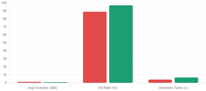
A condiment brand had been carrying two weeks of safety stock uniformly across all 32 active SKUs, regardless of velocity, variability, or margin contribution. High-velocity SKUs with predictable demand were overprotected. Seasonal SKUs with erratic demand were underprotected. After implementing dynamic safety stock calculated per SKU based on measured demand variability, lead time variability, and GMROI-based service level targets, total inventory reduced 23%, and service levels on the top 12 SKUs improved from 91% to 98%. The same working capital investment was simply redistributed to where it created the most value.
Integrating Production Constraints and MOQs
The theoretical replenishment model says order exactly what you need when you need it. The reality of CPG manufacturing says your co-packer requires 10,000-unit minimums, needs four weeks lead time, and can only produce your SKU during specific production windows. Balancing these realities against optimal order quantities is where replenishment modeling becomes genuinely complex.
The model needs to handle five production realities:
- Minimum order quantities change the ordering frequency calculation. If a co-packer requires 8,000 units and weekly demand is 2,200 units, the brand orders approximately every 3 to 4 weeks
- Production scheduling windows matter when co-packers run a SKU on a defined cycle. If the window is missed, the brand waits for the next one
- Shared component constraints arise when multiple SKUs use the same base ingredient or packaging, and evaluating combined ordering across those SKUs can hit volume thresholds for better pricing
- Capacity constraints during peak season require the model to prioritize production allocation across the SKU portfolio based on velocity, margin, and current inventory position
- Economic order quantity decisions involve evaluating whether ordering 12,000 units at $1.82 per unit makes more financial sense than ordering 8,000 units at $1.96 per unit, after accounting for the carrying cost of the additional inventory against the procurement savings
Channel-Specific Replenishment Logic
The biggest mistake brands make is applying the same replenishment logic across all channels. A grocery chain, a club store, a DSD convenience distributor, and an Amazon fulfillment center have fundamentally different replenishment requirements that a single model cannot address.
Channel Replenishment Requirements by Type
| Channel | Typical Pattern | Key Model Requirement |
| Grocery warehouse retailers | Weekly or biweekly, 5 to 10-day lead time | Forecast their next order date and size from the current WOS |
| Club stores (Costco, Sam’s) | Large quantities, quarterly intervals | Anticipate large orders without building inventory 3 months early |
| DSD convenience distribution | Continued to the distributor warehouse | Monitor distributor WOS, replenish to maintain a 3 to 4 week target |
| Food service distributors | Different seasonal patterns in retail | Separate seasonal indexing from retail channels |
| Amazon FBA and e-commerce | Continuous, 4 to 6 week check-in lag | Ship inventory well ahead to account for receiving delays |
For DSD distribution specifically, the model requires visibility into the distributor’s inventory position, not just the brand’s own warehouse. Replenishing your warehouse while the distributor sits on 9 weeks of supply creates a distorted demand signal and eventually results in returns or markdown requests. Replenishing when the distributor drops below 2 weeks of supply risks retail stockouts before the brand can respond.
Building Cash Flow Constraints Into Replenishment
This is where the CFO takes direct control of the replenishment model from operations. During periods of constrained cash flow, the model must integrate cash availability as a binding constraint on what gets ordered and when, not merely a consideration after the fact.
Available working capital defines the total purchase budget for the planning horizon. If $400K is available for inventory over the next month, the model cannot recommend orders totaling $650K, regardless of what the demand signal suggests.
GMROI-based prioritization determines which SKUs get funded when cash is constrained. A SKU generating 8x GMROI gets allocated working capital before one generating 2.5x GMROI, even if that means accepting a lower service level on the lower-return product.
Supplier payment terms affect the real cash impact of each order. If Supplier A offers net-60 terms and Supplier B requires net-30, ordering from Supplier A has a meaningfully different cash flow impact even when per-unit costs are identical.
Receivable timing allows the model to factor in incoming cash. If a $200K retailer payment is expected next week, that cash can be incorporated into replenishment decisions, potentially enabling orders that the current cash position alone would delay.
Implementation: 7 Practical Steps
Building this model requires integrating data from multiple systems and creating automated workflows that update daily. Here is the implementation sequence used with clients.
Step 1: Establish Data Infrastructure: Connect POS data from retailer portals or syndicated data providers such as IRI or SPINS. Integrate inventory positions from your 3PL or WMS. Link production schedules from your co-packer. Pull payment terms and lead times from your procurement system.
Step 2: Build the Demand Forecasting Engine: Use 24 months of historical POS data to establish baseline demand by SKU. Calculate monthly seasonal indices. Identify and quantify promotional lift patterns. Create the rolling 16-week forecast that updates automatically as new POS data arrives each week.
Step 3: Calculate Dynamic Safety Stock by SKU: Measure demand variability and lead time variability for each SKU. Set target service levels by SKU based on velocity, margin contribution, and strategic importance. Calculate dynamic safety stock and update the parameters monthly.
Step 4: Define Reorder Points and Order Quantities: For each SKU, calculate the reorder point as demand during lead time plus safety stock. Determine order quantities considering MOQs, production scheduling windows, and economic order quantities. Build channel-specific variants where needed.
Step 5: Integrate Cash Flow Constraints: Build rolling cash flow projections showing available working capital for inventory investment over 30, 60, and 90 days. Create GMROI rankings to prioritize SKUs during constrained periods. Establish override rules for strategically critical SKUs.
Step 6: Automate Daily Recommendations: Run the model daily, comparing inventory positions against reorder points, evaluating production schedules, checking cash availability, and generating specific purchase recommendations with order quantities and recommended ship dates.
Step 7: Establish the Review Cadence: Weekly review of forecast accuracy and whether model recommendations are being followed or overridden. Monthly recalibration of safety stock parameters and seasonal factors. Quarterly evaluation of service levels and inventory turnover versus plan.
Common Implementation Mistakes
After implementing replenishment models for dozens of CPG brands, the same mistakes appear repeatedly.
Forecasting from Shipments Instead of POS Data: Shipments to retailers are not consumer demand. They are a lagging indicator distorted by promotional timing, forward buying, and distributor ordering patterns. A brand loading the channel during a promotion will see shipment data show strong growth while actual consumer takeaway is flat. Always build forecasts from POS data when available.
Using Flat Safety Stock Rules Across All SKUs: Two weeks of safety stock on everything ignores the fact that different SKUs have different demand variability, different lead time reliability, and different strategic importance. Dynamic safety stock per SKU based on measured variability is not optional. It is the difference between the model working and it consistently failing.
Ignoring the Demand Decay After Promotions: A promotion generating 3x lift during the promotional week creates a demand trough the following week as consumers work through pantry inventory. The model must account for both the lift and the decay. Failing to model the decay leads to over-ordering for the weeks after a promotion ends.
Running Replenishment Separate from Cash Flow Planning: Operations ordering based purely on demand forecasts without visibility into cash availability is one of the most reliable ways for a fast-growing CPG brand to create a working capital crisis. The CFO must have direct input into which SKUs get funded and in what sequence during constrained periods.
Building the Model Once and Not Recalibrating It: A replenishment model built when the business had 15 SKUs and three retail partners needs significant recalibration when it grows to 40 SKUs and 12 retail partners. Seasonal factors shift. Demand variability changes. Co-packer lead times evolve. Monthly recalibration of safety stock parameters is not optional maintenance.
Optimizing for Service Level Without Considering GMROI: A 99% service level on every SKU sounds like an operations win until you calculate how much working capital is tied up in low-margin, slow-moving SKUs generating 1.8x GMROI. Strategic service level targets based on financial contribution, not just volume, produce meaningfully better returns on the working capital invested in inventory.
FAQ
How much historical data do I need to build a replenishment model?
You need minimum 12 months of POS data to understand seasonality, though 24-36 months is better for establishing stable seasonal patterns and variability measures. If you’re a new brand without historical data, you can use category benchmarks and competitive data as a starting point, then calibrate as your own data accumulates.
What if my retailers won’t share POS data?
Start with syndicated data from providers like IRI or SPINS, which cover major retailers. For retailers where POS isn’t available, use your shipment data but apply adjustment factors based on known channel inventory levels and estimated sell-through rates. The model will be less accurate but still better than pure gut feel.
How do I handle new product launches without historical data?
Use analogous item analysis. Find existing SKUs in your portfolio or competitive SKUs with similar price points, package sizes, and positioning. Use their velocity patterns as a baseline, adjusted for the specific characteristics of your new product. Update forecasts aggressively in the first 12 weeks as actual data becomes available.
What software or tools are required?
The model can be built in Excel/Google Sheets for brands with fewer than 30 SKUs and straightforward distribution. Beyond that, you’ll benefit from dedicated inventory planning software or building custom models in Python/R that can handle larger data sets and more complex optimization logic. Many brands start in spreadsheets and migrate to dedicated tools as complexity increases.
How often should the model run?
The forecast should update weekly as new POS data arrives. Replenishment recommendations should generate daily, checking inventory positions against reorder points and production schedules. Safety stock parameters should recalibrate monthly. Seasonal factors and service level targets should review quarterly.
What if my co-packer can’t meet the recommended production schedule?
The model needs to work within real-world constraints. If your co-packer can only produce your SKU every four weeks, build that constraint into the model and adjust order quantities accordingly. The goal is optimal decisions within actual constraints, not theoretical perfection that ignores reality.
How do I determine appropriate service level targets by SKU?
Start with velocity and margin contribution. Your top 20% of SKUs by revenue that also generate strong GMROI should target 97-99% service levels. Middle-tier SKUs might target 93-96%. Slow movers with marginal contribution can operate at 88-92%. Adjust based on strategic importance and retailer requirements.
What inventory turnover should I target?
It varies by category and business model. Most CPG brands should target 6-12x inventory turnover depending on shelf life, production economics, and distribution model. Faster turnover frees working capital but might increase per-unit costs due to smaller, more frequent production runs. The model helps you find the optimal balance for your specific situation.
How do I handle seasonality for products with limited history?
Use category-level seasonal indices from syndicated data as a starting point. If you’re launching a better-for-you snack bar, use seasonal patterns from the broader snack bar category. Adjust based on any unique characteristics of your product. After one full year, you’ll have your own seasonal data to refine the model.
What’s the ROI timeline for implementing a replenishment model?
Most brands see measurable improvements within 60-90 days. Initial benefits come from reducing expedited freight and catching obvious overstock situations. The full impact on inventory turnover and working capital reduction typically materializes over 6-9 months as you work through existing inventory positions and rebalance the portfolio.
